In this post I will attempt to explain the theory behind two-wheels self-balancing (TWSB) robot as clearly as possible. This post is not about the instruction or process of building such a robot, for this please refer to an earlier post here , where I discussed the micro-controller board that I used, the embedded software structure, and many other resources online. For videos of all robots made by me, please see https://www.youtube.com/fkungms.

1.0 The Basic Principle

Figure 1-1 - An inverted pendulum system.

Figure 1-2 - Action of the motorized cart when the inverted pendulum falls toward the front and back, in keeping the pendulum upright.
By reducing the motorized cart into just a pair of motorized wheels, we obtain a two-wheels self-balancing machine, as illustrated in Figure 1-3. From now on we will use the term TWSB Robot to refer to such machines.

Figure 1-3 - Converting the inverted pendulum platform into a two-wheels self-balancing machine.
2.0 High Level System Overview

Figure 2-1 - Basic building blocks of TWSB robot.

Figure 2-2 - Electrical connection of the key components.
3.0 Mathematical Model of the Robot Platform

A) The Main Body, which consist of the body and the two stators of the electric motor.
B) The Wheel Assembly, which consist of the wheel and the rotor of the electric motor.
If the electric motor contains gearbox, the gears, axles etc are part of the Wheel Assembly while the brackets for the gears, bearings would be part of the Main Body. Figure 3-2 shows a diagram of a TWSB robot and the division of the robot platform into Main Body and Wheel Assembly. We imagine the electric motor can be disassembled, one part goes to the wheel and another part stays with the body. Thus, in Figure 3-1, mb is the sum of the mass of the body and the two stators, similarly Jw is the moment inertia of the rotor and the wheel, reference to the center axis of the wheel.

3.1 Equations of Motion for the TWSB Robot

For one Wheel Assembly:

Figure 3-4A - Dynamic equations for the Wheel Assembly.
Main Body:

Figure 3-4B - Dynamic equations for the Main Body.

Figure 3-5 - The two equations of motion for the TWSB robotic platform.
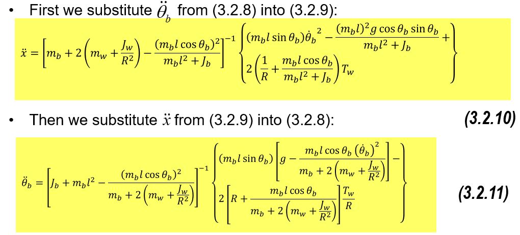
Equations (3.2.8) and (3.2.9) can be rewritten in the following form.
Figure 3-6 - The two equations of motion after some algebraic manipulation.
Extra Note: Couple moment, torque and reaction torque on an electric motor


3.2 Linear Equations of Motion for TWSB Robot
The equations of motion in (3.2.10) and (3.2.11) are non-linear, due to the presence of sine, cosine and square operations in the equations. Most of the time under normal operation the robot will be close to upright position, the rocking or rotation motion along the wheel axis small, i.e.:


4.0 The Complete TWSB Robot Model
4.1 Linear Model for Geared DC Motor
Working Principle of Geared DC Motor
Figure 4-1 - Model of geared DC motor.

Geared DC Motor Input-Output Relation
Using Kirchoff's Voltage Law, equations (4.1.1) and (4.1.2), the terminal voltage Va(s) across the rotor can be written as:

Because there is a gearbox between the motor and the output shaft, with gear ratio NG, the angle and torque relationship between the output shaft and motor are given by:


One final detail, because the motor enclosure or stator is not fixed, but free to rotate about the wheel axis, we also need to take this into account. Now as stated in Figure 4-2, thetam is the relative angle between the motor shaft (or Rotor) and enclosure. Since the motor enclosure can rotate, equation (4.1.5) needs to be modified as:

In most small DC gear motors, we can ignore the friction loss (DG is 0). Also impedance of the rotor inductance is small compare to the resistance, sLa << Ra. Hence the approximate form for geared DC motor input output relation, in frequency-domain is given by:


4.2 TWSB Robot Model with Geared DC Motor
When the geared DC motor is connected to the wheel, the angle of the motor shaft is equal to the wheel angle, and is related to the coordinate (x,0) of wheel axis. If we refer back to Figure 3-4A, using equation (3.2.3) and the fact that the motor shaft and wheel axis is connected via gearbox:


Scilab Software

Example 2 - Modeling a Small TWSB Robot
In this example we consider a small TWSB robot, using the motor described in Example 1. The Scilab scripts to calculate all the elements in the A, B, C, D matrices in the CLSS block is shown in Listing 1.
Listing 1 - Scilab script to calculate the Continuous Linear State-Space (CLSS) block representing the TWSB robot.
g = 9.8067; // m/s^2 - Acceleration due to gravity.
// Model parameters of TWSB Prototype.
// --- Parameters of Geared Motor ---
// From the datasheet of Pololu's 100:1 HP micrometal gear motor
Tstall = 0.0216; // N-m - stall torque in Kg/m.
RPMnoload = 320; // No-load RPM at Vin=6V.
wnl = (RPMnoload*2*%pi)/60; // No load gearbox output shaft rotation velocity in rad/sec.
Inl = 0.06; // No load current into motor, from measurement.
Vin = 6; // Volt. Input voltage to armature during test.
Istall = 1.6; // Amp, stall armature current.
Ng = 100; // Gear ratio.
Dg = 0.00001; // kgm/rad/sec - Viscous loss of gear.
La = 0; // Assume armature inductance is 0.
Ra = Vin/Istall; // Armature resistance.
Kt = (Tstall/(Vin*Ng))*Ra; // Armature torque constant.
Kb = (Vin-Ra*Inl)/(wnl*Ng); // Armature back EMF constant.
// --- Parameters of Motor Driver ---
Kmd = 1.0; // Voltage gain of motor driver (This depends on the implementation of the motor
// driver,
// --- Parameters of Wheel Assembly ---
R = 0.035; // m - Radius of wheel, 35 mm.
mw = 0.0343; // kg - Mass of wheel.
Jw = 0.5*mw*R*R; // kgm2 - Moment inertia of wheel assembly with reference to the center (axle).
// Here we can assume uniform mass distribution for the wheel and the rotor,
// then work out the respective moment inertia of the wheel and rotor separately.
// The effect of gearbox is ignored. Subsequently we add together
// the moment inertia for the wheel and rotor to get the approximate moment intertia
// for the wheel assembly. See any mechanics or physics texts on rotational dynamics.
// --- Parameters of Main Body ---
mb = 0.2445; // kg - Mass of the body and motor stators.
lb = 0.035; // m - Distance of center of mass to wheel axle.
Jb = 0.85*mb*lb*lb; // kgm2 - Moment inertia of Main Body reference to the center of mass.
// This is approximate only.
// Approximate constants for DC motor, gear box and wheel.
Cm1 = Ng*Kt/Ra;
Cm2 = Cm1*Kb;
M = mb + 2*(mw+Jw/(R*R)) - ((mb*mb*lb*lb)/(mb*lb*lb + Jb));
J = (mb*lb*lb) + Jb - ((mb*mb*lb*lb)/(mb + 2*(mw+Jw/(R*R))));
C1 = (1/M)*((mb*mb*lb*lb*g)/(Jb + mb*lb*lb));
C2 = (2/M)*((1/R) + ((mb*lb)/(Jb + mb*lb*lb)));
C3 = (mb*lb*g)/J;
C4 = (2/(J*R))*(R + ((mb*lb)/(mb + 2*(mw + Jw/(R*R)))));
// The elements of the state-transition (A) matrix
a11 = 0;
a12 = 1;
a13 = 0;
a14 = 0;
a21 = 0;
a22 = -C2*Cm2/(R*Ng);
a23 = -C1;
a24 = C2*Cm2;
a31 = 0;
a32 = 0;
a33 = 0;
a34 = 1;
a41 = 0;
a42 = C4*Cm2/(R*Ng);
a43 = C3;
a44 = -C4*Cm2;
// The elements of B matrix
b11 = 0;
b21 = C2*Cm1*Kmd;
b31 = 0;
b41 = -C4*Cm1*Kmd;
A few points need to be clarified in the Listing 1 on the physical parameters. The mass of the body, wheels, rotors and stators can be measured using small electronic scale. In the case of the DC motor, the motor is carefully dismantled to measure the mass of the rotor and stator (also the diameter of the rotor), then put back together again. The center of mass of the Main Body can be estimated using the bi-filar method, where we hang the Main Body at two positions using a thin thread or fishing line. The two positions must lie at the plane which divide the Main Body equal into right and left halves. The idea is shown in Figure 4-5.

Figure 4-5 - Dismantling the DC motor and measuring the CM of the main body.
5.0 Control and Balancing the TWSB Robot: State-Feedback Control
Now we are ready to implement a feedback control system to balance the TWSB upright. A direct way to do this is shown in the block diagram of Figure 5-1. This method of feedback control is usually called the State Feedback Control [2] because instead of feeding back a single parameter, we are feeding back an array of parameters representing the current state of the system, and applying a control parameter to each.
Figure 5-1 - State-feedback control of the TWSB robot with geared DC motors.
Compare to classical feedback control system, the state feedback control system shown in Figure 5-1 is a MIMO (Multi-Input Multi-Output) system. The input is the User Set Vector, and the output is the State Vector, which contain 4 elements. In contrast classical feedback control system is typically SISO (Single-Input Single-Output). In Figure 5-1 the feedback controller is simply a matrix multiplier, which multiply each element of the Error Vector with a coefficient. For instance coefficient kx multiply with the position error, kv multiply with linear velocity error and so forth. Of course the coefficients have to be selected carefully so that the TWSB robot can balance properly.
Assuming the system in Figure 5-1 is feasible or controllable, many techniques can be used to find the 4 feedback control coefficients kx , kv , ktheta and komega. For instance the most direct approach is trial-and-error or experimental method, where we try different combinations of the feedback control coefficients until satisfactory system response is obtained! There are some rules to systematically arrive at the values of the coefficients experimentally which I will summarize in Section 5.5. There are also a few analytical methods to find the feedback control coefficients, for instance a method called Pole Placement in control theory [2], see also this tutorial https://www.youtube.com/watch?v=M_jchYsTZvM&t=663s. In this method the coefficients are chosen such that the system exhibit poles and zeros in the complex plane that produce satisfactory time-domain behavior. Another popular method, the Linear Quadrature Regulator (LQR) [3] is based on computer optimization, where the coefficients are chosen such that a cost function that is based on the error vector, the control signal (vc) and any other parameters of interest is minimized. The cost function has a mathematical form called the quadrature form (whose output is always positive), thus the name of the method. Check out this tutorial on LQR method https://www.youtube.com/watch?v=1_UobILf3cc&t=419s. Demonstration of using LQR method and pole placement method to find the feedback control coefficients will also be shown in the Appendix.
In order to for the TWSB robot to balance upright, the user set vector can be set as in Figure 5-2. Basically this means we want the robot to remain upright (thetab = 0) without rocking back and forth, and also to remain stationary at the same location (x = 0).

Figure 5-2 - User set vector for the TWSB robot to balance upright and remain at same location.
Based on the TWSB robot model in Example 2, I created a complete Scilab XCOS model of the TWSB robot with state feedback controller as depicted in Figure 5-3.

Figure 5-3 - Scilab XCOS model of the TWSB robot with state feedback controller.
Of course in Figure 5-3, it is assumed that there are sensors to measure the state vector elements such as the tilt angle, tilt angle angular velocity, linear position and linear velocity. Also note that the user setting is a step function.
5.1 Some Computer Simulation Results with State-Feedback Control
Here we run a few simulations with different combination of the feedback control coefficient values. Figure 5-4A and 5-4B show the setting of the blocks in the Scilab XCOS model for the TWSB robot. The idea is to inject a small step disturbance to the user setting and see if the TWSB robot can remain in upright position for each set of feedback control coefficients.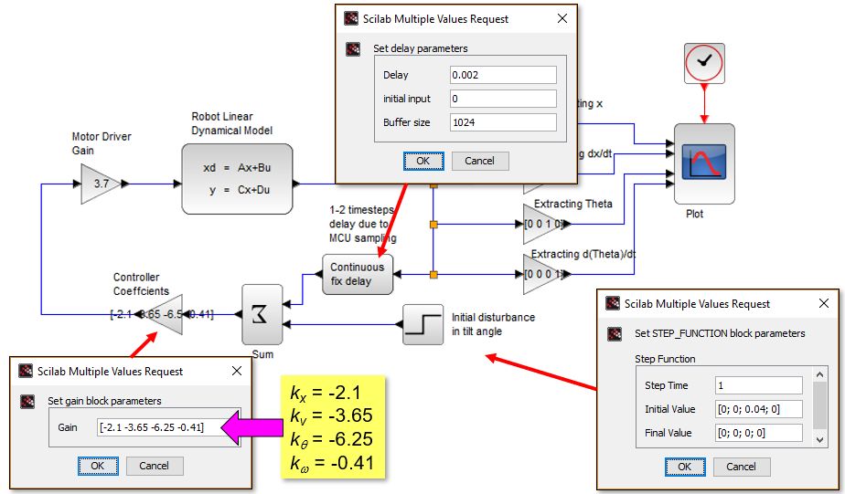
Figure 5-4A - Setting of the blocks for the TWSB robot with state feedback controller.

In Figure 5-4A the robot is initially set to tilt angle 0.04 rad at time t = 0.0, then at time t = 1.0 second the tilt angle is abruptly set to 0.0 rad, with all other set parameters remain at 0.0. The sequences of figures below illustrate the result of stable, not-so-stable and unstable feedback control coefficient values. The stable coefficient values are arrived at experimentally using the method described in Section 5.5. The not-so-stable coefficients result in a TWSB robot platform that requires drift longer distance on the ground and take longer time to reach the final state.

Figure 5-5A - Simulation results for stable feedback control coefficients.

Figure 5-5B - Simulation results for not-so-stable feedback control coefficients.

Figure 5-5C - Simulation results for unstable feedback control coefficients.
Here is a video of an example of TWSB robot using state-feedback control:
5.2 Special Case 1: Degenerating into PID Feedback Control
Although the linear mathematical model of the TWSB robot contains 4 parameters in the state, in principle we can still balance the robot upright by just focusing on the tilt angle and ignore the rest of the state parameters like x and dx/dt. This is illustrated in Figure 5-6. Because there is only one input parameter (thetab(set)) and one output parameter (thetab), this becomes a classical feedback control system (single-input single-output or SISO). Here we perform further operations on the error signal to obtain the differential and integration terms, and used PID controller to balance the robot upright. Although this will work, the dynamical performance of the TWSB robot will not be good generally compare to state-space feedback control. Because we ignore the position (x) and velocity (dx/dt), the robot will 'drift' a lot while balancing upright, and it is sensitive to disturbance such as when you knock into the robot, it will move about erratically.
Figure 5-6 - Ignoring all state parameters except for tilt angle, we can then use PID feedback control.
We can derive the transfer function for the robot when only focusing on the tilt angle error as shown in Figure 5-7. Here to be more realistic I also include the dead-band effect of the DC motor driver into the model. The coefficients of the PID controller can be determined analytically (say using Bode plot or Root Locus method) or experimentally. Here I arrived at the coefficients experimentally, first by tuning Kp, then Kd until the robot can balance, and finally Ki to reduce the drifting.

Figure 5-7 - Scilab XCOS model when ignoring all state parameters except for tilt angle, with PID feedback control.
Again we run the computer simulation from 0 to 15 seconds. The results are shown in Figure 5-8. Notice that because we do not take into account the state parameters x and dx/dt, the robot drifts about the floor while it is balancing upright, first x goes to almost 1 meter from the initial location, then gradually moves backwards until x becomes negative. We can reduce this drifting by tuning the default tilt angle thetab setting. However, generally using PID feedback control, it is very difficult to achieve zero drift, i.e. making the robot return to its original location.

Figure 5-8 - Simulation results for PID feedback control.
Here is a video of an example of TWSB robot using just PID feedback control, notice that the robot is sensitive to collision with objects, especially at the end of the video when the robot toppled over:
5.3 Special Case 2: TWSB Robot Using Brushless DC motors or Stepper Motors (Updated 2nd Sep 2021)
- Both types of motors do not use commutator and
- Both types of motors require external switching circuit or driver module to switch the direction of the electric current in the electromagnet (on the stator) in order to rotate.
- The rotational speed of both types of motors is proportional to the switching circuit frequency.
- The torque produced by both type of motors is more or less constant at low rotation speed. Typically the driver module uses a current source to drive the electromagnet in the stator, rendering the output shaft torque of the motor having constant average value at low rotation speed (when back EMF effect is small).
In principle we can derive a mathematical model of the brushless DC motor and stepper motor, as can be found in some literature, (see [4], [5]), and proceed as in the brushed DC motor case by putting the expression in equations (3.2.17a) or (3.2.17b) to obtain the final state equation of the TWSB robot with multiple inputs, say the supply voltage to the armature, the frequency of the switching circuit and other inputs. However here I will be using a different approach. This approach will be simpler but it is a less accurate model, which is fine as in practice we usually use computer simulation to guess the initial values of the feedback control coefficients and then arrive at the final values through experimentation. I will just focus on stepper motor and the case for brushless DC motor will be similar.
Here I will assume the stepper motor will be rotating at small angular velocity and that the output shaft is directly connected to the wheel without any gearbox. The former assumption is reasonable when the TWSB robot is close to upright position, the stepper motors will just rotate slowly clockwise or counter clockwise to keep the robot upright. At slow rotation the output torque from the stepper motors will be maximum and will be sufficient to propel the robot forward or backward. With this in mind let us consider equations (3.2.15) and (3.2.16) in frequency-domain form:


Assuming non-slip motion, the velocity of the TWSB robot and the wheel angular velocity are related to the wheel radius R:


Figure 5-9 - Scilab XCOS model for TWSB robot using stepper motors for propulsion with velocity as input control.
A straight forward approach to map the PID controller output to the wheel angular velocity is to control the frequency of the periodic pulse signal used to drive the stepper motor driver modules (the block "Stepper Motor Driver Gain" in Figure 5-9 encompasses this relationship). A stepper motor is driven by pulse, each pulse will rotate the motor shaft by a fixed angle clockwise or counter-clockwise. This fixed angle is called the Step Angle qstep and can be set by the user. Typical values for step angle is 1.8 degree for full-step, 0.9 degree for half-step. As an illustration, assuming we are using bipolar stepper motor under half-step mode, 400 pulses will be needed to drive the motor shaft one rotation (360/0.9 = 400). If a rotation speed of 0.5 rotation/second, or 3.142 radian/second is needed, we would need to send 200 pulses to the stepper motor driver every second, or a frequency of 200 Hz. Thus, the stepper motor rotation speed is given by qstep/T. where T is the period of one pulse. The PID controller output must be mapped to the correct value of T for the stepper motor to turn at the required angular velocity as shown in equation (5.3.6).

Because of the inversely proportional relationship between stepper motor angular velocity and T, we need to use a non-linear function to relate T with PID controller output. Any point to note is since we are going to generate the control pulses using digital hardware, the value of T will be discrete, some values of T cannot be synthesized and need to be approximated to the nearest value supported by the hardware. A typical relationship that is popular for mapping PID controller output to stepper motor driver is shown in equation (5.3.7):

In equation (5.3.7), Δt
is the time resolution, it is dependent on the micro-controller
hardware such as the timer resolution, clock frequency etc, with typical
value of 5-50 micro-seconds. The parameters a and b are set by the user to adjust the slope or gain of the PID Controller versus stepper motor speed curve. For example if you are using Arduino Uno (with Atmega 328P micro-controller) running at 16 MHz clock frequency (0.0625 micro-second per cycle), it will be impossible to have Δt less than 10 micro-seconds as you would not have enough clock cycles to execute other codes for the robot controller.
A mapping example is shown in Figure 5.10 below for qstep = 0.9 degree, Δt = 20 microsecond, a = 4000, b = 3, with PID Controller output capped to between -400 to +400. Due to the need to cast the PID Controller output to integer (because the pulse generator requires integer input to it's timing registers), the mapping exhibits nonlinear steps as indicated in Figure 5-10. Hence, the user should set the mapping function carefully to minimize the nonlinear steps within the typical wheel velocity range.

Figure 5-10 - Mapping of PID Controller output to wheel angular velocity with a slope around 0.4.
With the model in Figure 5-9, we can use standard analytical method in control theory to obtain the coefficients for the controller, or we can simple do it via trial-and-error. A sample result for the model in Figure 5-9 is shown in Figure 5-11. Similar to the idea in Section 5.1 and Section 5.2, where initially we assume the TWSB robot to be upright, then we inject a small step change in the user setting. If the system is stable the TWSB robot should be able to regain balance with some changes in it's dynamic parameters. In Figure 5-11 the user settings is changed from 0 degree to 2 degree at t = 3.0 seconds. We observe that the stepper motor based TWSB robot regain balance after 1.0 second. However to remain upright at body tilt angle of 2 degrees, the TWSB robot has to continuously accelerate at roughly 0.6 m/s^2. Thus the robot will keep on moving faster and faster until it topples over, unless we reduce the user settings. More detailed explanation can be found in this paper.

Figure 5-11 - Scilab XCOS simulated results when user setting is changed from 0 to 2 degrees.
Videos, Design Files and Codes
Here is a video of an example of TWSB robot using NEMA 17 stepper motors, with PID feedback controller setting the rotation velocity of the stepper motor shaft. You can see the design details here. Note that I am not using Arduino for this particular build.
It is also possible to write equation (5.3.3) in state-space form, using the phase variable approach [2], this is illustrated below. However, since we have only one 2nd order system equation in the case of stepper motor, the state matrix for the robot is a 2x2 square matrix, i.e. only 2 parameters are needed to determine the system state. First we define two new state parameters:

Then we modify (5.3.3) using the parameters above:

This can then be rewritten in matrix form:

State-feedback control method as described in Section 5.1 can then be applied to equation (5.3.5) to keep the robot platform upright.
5.4 Non-Ideal Effects
In coming up with the control schemes in previous sections we have made some assumptions. First and foremost is the fact that the perturbation of the robot platform from the required state is small and the dynamical equations constraining the robot platform behavior can be linearized. The second important assumption is that we can measure all the physical parameters such as the tilt angle thetab, d(thetab)/dt, x and dx/dt accurately and without any time delay. Thirdly any non-linearity effects in the motor, motor driver circuit are ignored. Typically there will be some error and delay in estimation of the state vector of the robot platform due to the way the sensors work, noise and the algorithms used, for example the Kalman Filter and Complementary Filter approaches are usually used to obtain an estimate of tilt angle thetab, d(thetab)/dt from the accelerometer and gyroscope. Also the micro-controller can take a few tens to hundreds of micro-seconds to perform all the calculations. Finally there are non-linear frictional force in the motor and gearbox, and saturation effect in the motor driver circuit. All these can be modeled mathematically and included in our Scilab XCOS model to give a more realistic prediction of the robot platform behavior.
5.5 Some Suggestions for Tuning the State-Feedback Coefficients (Updated on 11 July 2021)
- First set kx , kv , ktheta , kw and thetab(default) to 0. Use a support to hold the robot upright.
- Slowly increase (or decrease) ktheta until the robot oscillate around the upright position. The polarity of ktheta should be such that when the robot tilts forward, the wheels should be driven to move the robot forward, vice versa when the robot tilts backward.
- Slowly increase (or decrease) kw until the robot can balance briefly. The robot will move or drift when it is attempting to balance upright because kx and kv are still 0.
- Now adjust kx and kv until the robot can balance without drifting a lot. From experience kx and kv usually have similar polarity and are negative. Coefficients kx and kv affects the dynamic response of the robot when it is pushed, so once the initial kx and kv are obtained to stop the robot from drifting, we should tune these coefficients to optimize the dynamic response when disturbed. Typically, this is done by observing the plot of velocity and distance traveled versus time when the robot is pushed. A properly tuned kx and kv should allow the robot to gradually return to the initial position. Adjust kx and kv to reduce overshoot/undershoot in the robot movement when pushed and to achieve the best damping ratio.
- Finally tune thetab(default) by putting the robot upright (with the motors not running), and then activating the balancing routine. If thetab(default) is not right the robot will drift a short distance when balancing routine is engaged. thetab(default) should be tuned until the robot can ‘stands’ and balance at the starting location without too much movement when balancing routine is engaged.
- Deadband correction for motor driver - Typically we need to add an offset voltage to the motor driver board, to overcome the internal friction of the motor, gearbox and the wheels. This value can be discovered experimentally by trial-and-error. With the correct offset voltage, the robot will have minimum rocking motion while balancing at a location.
- Optimizing the dynamic response to disturbance - After completing step 1-6, the robot should be able to balance on two-wheels quite well. We can now improve it’s balancing ability further by optimizing the 4 control coefficients kx , kv , kp , kw and b(default). One of the interesting observation is this, if the coefficient corresponding to a parameter is not optimum (say too small), then when the robot is disturb, say be pushing it, then that particular parameter will exhibit large disturbance. An example if coefficient kw which corresponds to db(default)/dt has a magnitude that is too small, the robot can balance on two-wheels. But when pushed, it will rock to front and back while remaining almost stationary at same location x. Thus if the magnitude of kx is too small then the robot will drift. And if magnitude of kv too small, the robot will move back and forth when pushed. But pushing the robot platform and continuous carrying out small adjust to the values of the control coefficients, when can arrive at a set of coefficients that will give a robust robot dynamics.
6.0 The Next Step
The steps described in this article are just to allow the robotic platform to balance reliably on two-wheels. To have the TWSB work, we need to make it perform higher order motions, such as move at constant velocity in a preset direction, turning, tackling slope or incline surface, going through small obstacles, carrying loads etc. This entails further refinements to the algorithms presented here. Probably I will write another article to describe these refinements. For some interesting videos, please see this channel.
References
- F. Grasser, A. D’Arrigo, S. Colombi, A. C. Rufer, “JOE: A mobile, inverted pendulum,” IEEE Transactions on Industrial Electronics, vol. 49, no. 1, pp. 107-113, 2002.
- N. S. Nise, "Control systems engineering", John-Wiley, 6th edition, 2011.
- G. F. Franklin, J. D. Powell, M. Workman, "Digital control of dynamic systems", Pearson (Addison Wesley), 3rd edition, 1998.
- B. C. Kuo, G. Singh, R. Yackel, "Modeling and simulation of a stepping motor", IEEE Transactions on Automatic Control, Vol. 14, No. 6, 745-747, 1969.
- A. Morar, "Stepper motor model for dynamic simulation", Acta ElectroTehnica, Vol. 44, No. 3, 117-122, 2003.
- F. P. Beer, E. R. Johnston Jr., E. Eisenberg, W. Clausen, P. J. Cornwell, "Vector mechanics for engineers - Dynamics", McGraw-Hill, 8th edition, 2006.
Appendix 1 - Controllability of TWSB Robot Model
Test for controllability of a linear system in state-space form can be done by checking the Rank of the Controllability Matrix CM. For an nth order system, if the rank of CM is also n, then the linear system is completely controllable [2]. Matrix CM is given by:

Figure A1-1 - The controllability matrix.
Thus for TWSB robot model, the rank of the CM must be 4 in order to be completely controllable. Scilab has built-in library to compute CM in the form of the cont_mat( ) function. Please refer to the online help of Scilab for further details.
Appendix 2 - Using Pole Placement and LQR Method to Find the Coefficients for State Feedback Control
Scilab also has built-in library for the pole placement and LQR algorithm in the form of the ppol( ) and lqr( ) function. In order to use these functions the state-space system must be controllable. Listing 2 below is a modification of the Listing 1 scripts, where I include the the controllability test and the steps to compute the feedback control coefficients using LQR algorithm, and also calculate the final values of all the poles in the closed-loop system. The script is created as a Scinote file and executed on Scilab console. The results are shown in Figure A2-1. As can be seen in Figure A2-1, the TWSB robot model with state-feedback has CM with rank of 4, thus completely controllable.
Listing 2 - Scilab script to calculate the Continuous Linear State-Space (CLSS) parameters representing the TWSB robot, and also to perform controllability test and calculate the LQR feedback control coefficients.
       g = 9.8067;             // m/s^2 - Acceleration due to gravity.

// Model parameters based on V2 Prototype.
// --- Parameters of Geared Motor  ---
// From datasheet of 100:1 HP micrometal gear motor
Tstall = 0.021602;       // N-m - stall torque (2.2 kg/m).
RPMnoload = 320;        // No-load RPM at Vin=6V.
wnl = (RPMnoload*2*%pi)/60;     // No load gearbox output shaft rotation velocity in rad/sec.
Inl = 0.06;             // No load current into motor, from measurement.
Vin = 6;                // Volt. Input voltage to armature during test.
Istall = 1.6;           // Amp, stall armature current.
Ng = 100;                // Gear ratio.
Dg = 0.00001;           // kgm/rad/sec - Viscous loss of gear.
La = 0;                 // Assume armature inductance is 0.

Ra = Vin/Istall;            // Armature resistance.
Kt = (Tstall/(Vin*Ng))*Ra;   // Armature torque constant.
Kb = (Vin-Ra*Inl)/(wnl*Ng);           // Armature back EMF constant.

// --- Parameters of Motor Driver  ---
Kmd = 3.16;             // Voltage gain of motor driver.

// --- Parameters of Wheel ---
R = 0.035;              // m - Radius of wheel, 70mm 3D printed wheels.
mw = 0.0343;            // kg - Mass of wheel.
Jw = 0.5*mw*R*R;        // kgm2 - Moment inertia of wheel reference to the center (axle).
                        // This is approximate only, assuming uniform mass distribution.
// --- Parameters of Robot Body ---
mb = 0.2445;            // kg - Mass of body.
lb = 0.035;             // m - Distance of center of mass to wheel axle.
Jb = 0.1*mb*lb*lb;     // kgm2 - Moment inertia of Body reference to the center of mass.
                        // This is approximate only.

// Approximate constants for motor, gear box and wheel.
// See the derivation, V3, 31 March 2017.
Cm1 = Ng*Kt/Ra;
Cm2 = Cm1*Kb;
M = mb + 2*(mw+Jw/(R*R)) - ((mb*mb*lb*lb)/(mb*lb*lb + Jb));
J = (mb*lb*lb) + Jb - ((mb*mb*lb*lb)/(mb + 2*(mw+Jw/(R*R))));
C1 = (1/M)*((mb*mb*lb*lb*g)/(Jb + mb*lb*lb));
C2 = (2/M)*((1/R) + ((mb*lb)/(Jb + mb*lb*lb)));
C3 = (mb*lb*g)/J;
C4 = (2/(J*R))*(R + ((mb*lb)/(mb + 2*(mw + Jw/(R*R)))));

// The elements of the state-transition (A) matrix.
a11 = 0;
a12 = 1;
a13 = 0;
a14 = 0;
a21 = 0;
a22 = -(C2*Cm2)/(R*Ng);
a23 = -C1;
a24 = C2*Cm2;
a31 = 0;
a32 = 0;
a33 = 0;
a34 = 1;
a41 = 0;
a42 = (C4*Cm2)/(R*Ng);
a43 = C3;
a44 = -C4*Cm2;
// From the A matrix.
A = [a11 a12 a13 a14;a21 a22 a23 a24;a31 a32 a33 a34;a41 a42 a43 a44];

// The elements of B vector.
b11 = 0;
b21 = C2*Cm1*Kmd;
b31 = 0;
b41 = -C4*Cm1*Kmd;
// Form the B vector.
B = [b11;b21;b31;b41];

C = eye(4,4); // Create a 4x4 identity matrix.

// Form the linear system model.
// x = Ax + Bu
// y = Cx + Du, where D = 0, u = input.
P = syslin("c", A, B, C);

// Perform controllability test.
CM = cont_mat(A,B);
disp('Rank of CM is:');
rank(CM)

// --- LQR Method to find feedback coefficients ---
// The cost function weights for LQR algorithm.
Q = diag([2.0 2.0 0.5 0.1]);    // Emphasize x, v errors, deemphasize theta and
                                // d(theta)/dt errors.
R = 2.0;                        // Emphasize control voltage magnitude.  We do
                                // not want a control voltage that is too big,
                                // prevent wastage of energy.
disp('LQR coefficients');
Klqr = lqr(P,Q,R)                 // Calculate the LQR coefficients.

// Finding the composite state transition matrix.
// Note: We can write as A - B*(-Kq)
Aux = A + B*Klqr;
// Finding the roots of the compensated system, e.g the eigenvalue of
// the composite state transition matrix.
disp('Poles of the closed-loop system using LQR');
spec(Aux)

// --- Pole Placement Method to find feedback coefficients ---
// Here we are assuming a percent overshoot of roughly 15%, and settling
// time of roughly 4.0 seconds. This would (see [2]) requires damping factor
// of 0.5 and natural frequency of 2.667 rad/seconds, and a dominant
// complex poles of
// P1, P2 = -1.333+j2.309 and -1.333-j2.309
// We also select the 3rd and 4th poles as real poles, sufficiently far away
// from the dominant poles. This would mean the 3rd and 4th poles should be at
// least 10x further away from the imaginary axis compare to the dominant poles.
// So we arbitraryly take P3 = -13.333 + j0 and P4 = -26.666 + j0
Real = -1.333;
Imaginary = 2.309;
p1 = Real+%i*Imaginary;
p2 = Real-%i*Imaginary;
p3 = -13.333;
p4 = -26.666;
disp('Pole placement coefficients');
Kpp = ppol(A,B,[p3, p4, p2, p1])
Aux2 = A - B*Kpp;
disp('Poles of the closed-loop system using pole placement');
spec(Aux2)

Figure A2-1, the state-feedback coefficients obtained using LQR method are:kx = -1.000
kv = -1.575
ktheta = -5.165
komega = -0.334
Note that we need to multiply the output of lqr( ) with -1 due to the polarity of feedback value to the summing network assumed by the Scilab lqr( ) function, which is positive instead of negative as in Figure 5-1. Comparing the values above with the coefficients used in Figure 5-4A and we can see that the coefficients above are within the same range.
Also from Figure A2-1, the state-feedback coefficients obtained using pole placement method are:
kx = -1.909
kv = -0.931
ktheta = -3.659
komega = -0.158
If we use both sets of state-feedback coefficient in our actual robot or in Scilab XCOS simulation as in Figure 5-4A,
can check that the system should be stable.
Thank you very much for your explanation.
ReplyDeleteI think equation (3.2.14c) has redundant theta-b.
Yes you are right, the theta-b should not be there, thanks for pointing out. Will correct later.
DeleteCan you provide some referene for Bifilar method of estimating centre of mass of main body or any other method?
ReplyDeleteAlso how to calculate momment of inertia of main body?
You have taken Jb = 0.85*mb*lb*lb in your code.. can you explain this approximation a little bit please?
For finding the center of mass, any college level physic textbooks that deal with mechanics should provide the concepts. For instance
Deletehttps://www.scientificamerican.com/article/x-marks-the-spot-finding-the-center-of-mass/
Maybe my definition of bifilar is different from what you have in mind.
For Jb, it depends on the shape of the robot body. You can use the Moment Inertia (MI) formula for a uniform rectangular object. I approximate the robot body as a few uniform rectangular objects (battery and circuit boards apart from main body), and combine them using parallel axis rule. Again this can be found in typical physics textbook. Of course you can use CAD software and these software can work out the more accurate estimation of center of mass and moment inertia reference to a certain pivot. For my case I find that Jb = 0.85*mb*lb*lb give reasonable approximation.
Hey, big thanks, Have you tried implement lqr method with stepper motor? I'm trying it, but it's so hard to do. Can you help me?
ReplyDeleteI haven't try LQR with stepper motor. But the robot equation with stepper motor can be written in state-space form to use with LQR and other matrix based feedback control methods. I've updated Section 5.3 to show how this is done. Note that the LQR loop is only to make the robot balance upright, to make the robot move at constant speed while balancing upright, you need to add another loop on top of the LQR loop.
DeleteHey,can you please explain what you mean by "adding another loop on top of the LQR loop? is it done by adding another pid controller?
DeleteYes run another PID controller 'on top' of LQR loop. The setpoint of the system (x1 x2) (see equation (5.3.4)) represents the tilt angle and it's rate-of-change. Normally (x1 x2) = (0 0) when we want to balance the robot. We can set (x1 x2) = (0.01 0) to move the robot forward, and (-0.01 0) to move the robot backward. You need to control this small offset or the robot will keep on moving faster and faster. So adding a feedback loop to do this automatically is called 'adding another loop on top'
DeleteHey, wondering if you had to deal with speed control fir the motors as well to account for motor difference?
ReplyDeleteEssentially similar to what is here https://medium.com/husarion-blog/fresh-look-at-self-balancing-robot-algorithm-d50d41711d58
DeleteYes I include speed and direction controls. I did not explain in the blog, but I include a link to a paper in blog that describes the details(see link just above Fig. 5-10) I have 3 control loops, the main control loop to balance the robot. Then two outer loops modulate the main loop to control direction and speed.
DeleteHey, thanks!
DeleteIs possible define a full space state form, like 4.2.2a, considering stepper motor dynamics?
I’m trying developing a lqr stepper motor. I alread did it with dc motor and encoder.
This comment has been removed by the author.
DeleteActually LQR or similar method can be applied to any system that can be expressed in state space form. Both 4.2.2a and 5.3.5 are examples of state-space form, just that the state parameters and input are different. LQR is just a method to find a set of feedback coefficients that will minimize a specific loss function, it's a form of optimization. Do read it up in books. If you also need to control the distance, can expand the 2x2 state transition matrix in 5.3.5 to include a 3rd variable, x3 which is related to the angle thetaw (the state transition matrix will then become 3x3). If you insist to cast the stepper motor platform into 4.2.2a form, yes in principle it can also be done. But it is not practical if you are using standard stepper motor driver IC to drive the stepper motor. Think of it, when you drive stepper motor, it is roughly either full torque or no torque, unlike brushed motor control where you can adjust the motor output torque to a fine degree.
DeleteHello from Argentina, thanks a lot for sharing this! I`ve seen in other resources (for exaplme this in page 734 https://sciendo.com/article/10.1515/ijame-2017-0046) that for the model of DC gearmotor equation 4.1.4a is not used, instead they apply Newtons 2nd law for rotation of the motor shaft resulting something like:
ReplyDeleteTm(s)=Jm*s^2*thetham + bm*s*thetham + TL(s)
Where Jm is motor inertia, bm es motor damping coeff and TL torque due to motor load. This is not used in your analysis.
Could you help me understand this difference?
For simplicity assume motor is connected directly to the wheel. I combine the motor's rotor with the wheel (I call it wheel assembly), and the stator with the body, see Fig 3-1 and Fig 3-2. So Jw in equation (3.2.2) combines wheel and rotor moment inertia, and mw includes the rotor mass. In between the body and wheel assembly is the complementary torque pair due to magnetic field interaction between the rotor and stator of the motor, and the constraint forces due to the bearing and the brackets. Also I ignore viscocity loss in the motor, e.g. bm=0. Thus, a logical way to separate the bodies is at the space between the rotor and stator of the motor.
DeleteAnother popular method to derive the system equations is using Lagrange-Euler equation (based on Hamilton's energy principle), which can be shown to be equivalent to Newtonian mechanics. I think there could be a minor omission in equations (2.5) & (2.6) in the paper you mentioned, the kinetic energy component of the rotor, stator and gearbox should be included. But the effect will be negligible if the motors are small in comparison to the total robot.
Hello I’m implementing an LQR for a two TWSB robot as well using and arduino and raspberry pi zero any tim on implementing the LQR on arduino and filtering the data from sensor
ReplyDeleteThank
Before your start tuning the LQR parameters, make sure the robot tilt angle estimation is accurate (compare to actual physical measurement). Sometimes the robot cannot balance is because the tilt angle estimation not good. I've tried both Complementary Filter and Kalman Filter method to estimate the tilt angle, both works well. Although KF can adapt to change in MEMS sensor.
DeleteHey, Isn't equation (5.3.5 )only for balancing the robot.Can you please explain in detail how to move and turn the robot while balancing?
ReplyDeleteYes (5.3.5) only for balancing the robot upright. To turn the robot, add a small differential offset to the wheel velocity value. For instance if you calculate that at instance t, you need to turn both wheels forward at 0.5 revolution/second, to keep the robot balance. To turn right, set right wheel velocity to 0.45 r/s, and left wheel to 0.55 r/s. Keep to 10% of the max rotation in your system. To move forward, instead of using [0, 0] as your setpoint (the 1st parameter is the body or tilt angle in radian, 2nd is the rate of change of the body angle in radian/sec), use [0.01, 0]. If you analyze the equation of motion as in Section 3, you will see that the machine needs to keep moving forward to main a positive tilt angle.
ReplyDeletehey,iam trying to code the lqr method with stepper motor in an Arduino board.I have calculated the K matrix.But how do i code the feedback?
ReplyDeletedo i need to multiply K with error(difference between body tilt angle and upright position) or multiply it directly with the current body tilt angle
Also what to do next after multiplying with K matrix ?
Yes multiply each element in K vector with the corresponding error, then sum up. The result is the voltage to apply to the motors. See Figure 5.1. For instance v = kx*ex + kv*ev + ktheta*etheta + kphi*ephi
DeleteThis comment has been removed by the author.
DeleteBut for the method of using stepper motors, in Figure 5-9 control signal is angular velocity of the wheels right ?
Deletei.e angular velocity of wheel = kthetaB*ethethaB+kthetaBdot*ethetaBdot
Also how can I map this control signal to the pulse rate required for driving the stepper motors.
Correct. The angular velocity of the wheel is proportional to the frequency of the control pulse. The exact mapping of the control signal to pulse rate depends on the stepper motor driver chip, the step setting of the chip (i.e. full step, half-step, or other micro-stepping scheme) and the step angle of the stepper motor. You can see the codes for many Arduino based project or the one I shared here for dsPIC33 micro-controller, under "Videos, Design Files and codes"
DeleteHey, I'm trying to make this robot using nema17 stepper motors with a4988 drivers, could you please tell me how you calculated the stepper motor driver gain of 0.55 for the Scilab simulation?
ReplyDeleteActually a bit complicated, I did describe it in the codes and also on the paper. Assuming that we use quarter-step mode to turn the stepper motor, the output of the PID controller will be scaled to an integer between -400 to +400. This value is then converted to rotation speed of the wheel in radian/second, and is dependent on the algorithm and the computer/micro-controller hardware. Basically the PID controller output will be map to frequency from a pulse generator that I implemented in the micro-controller, and this pulse is used to drive the stepper motor driver. You can find the details in the code. You can do an experiment to plot the rotation speed of motor versus the PID controller output and then approximate the gain. In my case, based on the pulse generator and some mapping formula (see explanation in codes), I use a spreadsheet to plot a graph of rotation speed versus PID value and then work out the slope.
DeleteHere's the extract from the paper I shared "• The output of the PID controller is converted into a periodic square wave using a hardware timer in the on-board computer. This periodic pulse is then used to drive the stepper motor driver IC. The Stepper Motor Driver Gain block after the PID controller in Fig. 6 accounts for the conversion between PID controller output and the actual angular velocity obtained using (1). This value of the gain block depends on the resolution of the hardware timer, the step angle of the stepper motor and the non-linear equation used to map the PID controller output to the timeout period of the hardware timer. It is hardware and algorithm dependent."
DeleteHey, thanks for this amazing article. Im going thru the equations and Im wondering if the theta dot squared factor in equation 3.2.11. should be negative?
ReplyDeleteYes you are right. The affect term vanish under linear approximation hence I did not detect it for so long. Thanks, have corrected in the post.
Delete